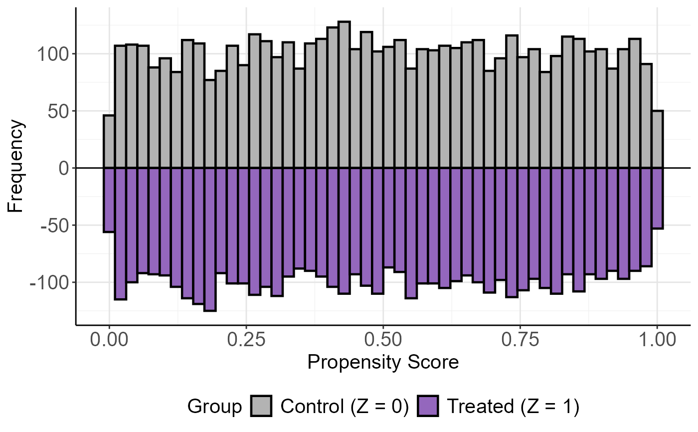
Mirror Histogram of Propensity Scores — mirror

Creates a mirror histogram to compare the distribution of propensity scores between treated and control groups introduced by Li and Greene (2013).

Usage

mirror_hist(
  object = NULL,
  ps = NULL,
  Tr = NULL,
  bins = 70,
  size = 0.5,
  theme.size = 15,
  grid = TRUE,
  ...
)

Arguments

object: An optional object of class `lbc_net`. If provided, extracts `ps` (fitted propensity scores) and `Tr` (treatment assignment).
ps: A numeric vector of propensity scores. Required if `object` is not provided.
Tr: A binary numeric vector indicating treatment assignment (1 for treatment, 0 for control). Required if `object` is not provided.
bins: Integer specifying the number of bins in the histogram. Default is 70.
size: Numeric specifying the line size for the histogram bars. Default is 0.5.
theme.size: Numeric specifying the base font size for the theme. Default is `15`.
grid: Logical indicating whether to include gridlines in the plot background. Default is `TRUE`.
...: Additional arguments passed to `ggplot2` layers for customization.

Value

A `ggplot2` object for further customization or direct display.

Details

This function creates a mirror histogram where the control group (Z=0) is displayed above the x-axis and the treatment group (Z=1) is displayed below the x-axis, making it easier to compare the distribution of propensity scores across groups.

Examples

# Example with manually provided propensity scores and treatment indicators
set.seed(123)
ps <- runif(10000)  # Simulated propensity scores
Tr <- sample(0:1, 10000, replace = TRUE)  # Random treatment assignment
mirror_hist(ps = ps, Tr = Tr, bins = 50, size = 0.8)


if (FALSE) { # \dontrun{
# Example with an `lbc_net` object
model <- lbc_net(data = data, formula = Tr ~ X1 + X2 + X3 + X4)
mirror_hist(model)
} # }