Purpose of This Example
This example demonstrates how to apply LBCNet on a simulated dataset inspired by the misspecified propensity score model from Kang & Schafer (2007). Our goal is to estimate the mean outcome, assess covariate balance, and evaluate propensity score calibration using local system Python.
Simulate the Data
We simulate data where the true propensity score model differs from the one used in the analysis, representing a challenging scenario for causal inference (misspecified propensity score model).
# Load required packages
library(MASS)

# Set seed for reproducibility
set.seed(123456)

# Define sample size
n <- 5000

# Generate true covariates from a multivariate normal distribution
Z <- MASS::mvrnorm(n, mu = rep(0, 4), Sigma = diag(4))

# Generate true propensity scores
prop <- 1 / (1 + exp(Z[,1] - 0.5 * Z[,2] + 0.25 * Z[,3] + 0.1 * Z[,4]))

# Assign treatment based on propensity scores
Tr <- rbinom(n, 1, prop)

# Generate continuous outcome (correct model)
Y <- 210 + 27.4 * Z[,1] + 13.7 * Z[,2] + 13.7 * Z[,3] + 13.7 * Z[,4] + rnorm(n)

# Create a set of covariates for estimation (misspecified model)
X <- cbind(
  exp(Z[,1] / 2),
  Z[,2] * (1 + exp(Z[,1]))^(-1) + 10,
  ((Z[,1] * Z[,3]) / 25 + 0.6)^3,
  (Z[,2] + Z[,4] + 20)^2
)

# Combine data into a data frame
data <- data.frame(Y, Tr, X)
colnames(data) <- c("Y", "Tr", "X1", "X2", "X3", "X4")

# Quick look at the data
head(data)
         Y Tr        X1        X2        X3       X4
1 267.0934  1 2.0995290 10.136751 0.1936739 465.4067
2 211.1973  1 1.0944490 10.811059 0.2031783 462.5301
3 190.5548  1 1.1113093  9.313208 0.2168326 327.9726
4 209.1748  1 0.9292040 10.001453 0.2145796 403.6159
5 198.9068  1 0.4234368 10.261615 0.2123729 508.9887
6 235.8486  0 0.7080015 11.445936 0.2109414 529.2390
Set Up Python Environment Using a Virtual Environment
In this example, we set up LBCNet to run in a Python virtual environment called "r-lbcnet".
Using a virtual environment ensures the Python packages needed for LBCNet are installed and isolated from other projects.
library(LBCNet)

# Set up LBCNet to use a virtual environment named "r-lbcnet"
setup_lbcnet(
  envname = "r-lbcnet",       # Name of the virtual environment
  create_if_missing = TRUE   # Set to TRUE if you want LBCNet to create the environment automatically if it doesn't exist
)
Here, envname = "r-lbcnet" specifies the name of the Python virtual environment and create_if_missing = FALSE means LBCNet will automatically create a new virtual environment and install the necessary Python dependencies (like torch) if it doesn’t already exist.
Fit the LBC-Net Model
Estimate propensity scores using LBC-Net with the covariates X1, X2, X3, X4, and then compute the causal estimator (Inverse Probability Weighting estimator) of ATE.
# Fit the LBC-Net model
lbc_net.fit <- lbc_net(
  data = data,
  formula = Tr ~ X1 + X2 + X3 + X4,
  Y = data$Y,
  estimand = "ATE"
)
Python is already set up. Skipping `setup_lbcnet()`.
Calculating propensity scores for ck/h calculation...
⚠️ Stopping criterion not met at max epochs. Try increasing `max_epochs` or adjusting `lsd_threshold` for better convergence.
Starting post-processing: computing treatment effect and variance...
✅ LBC-Net training completed successfully.
# Print the model fit object
print(lbc_net.fit)
Call: Tr ~ X1 + X2 + X3 + X4
Sample Size: 5000  | Treated: 2466  | Control: 2534
Estimand: ATE (Average Treatment Effect)

--- Training Results ---
Final Loss Value: 840.804
Max LSD: 3.92%
Mean LSD: 0.40%

--- Model Hyperparameters ---
Hidden Layers: 1 | Hidden Units: 100
VAE Learning Rate: 0.010 | LBC-Net Learning Rate: 0.050
Weight Decay: 1.0e-05 | Balance Lambda: 1.00
Kernel: "gaussian"

--- Stopping Criteria ---
LSD Threshold: 2.00% | Rolling Window: 5
Max Training Epochs: 5000

--- Treatment Effect (stored in object) ---
Estimand: ATE (Average Treatment Effect)
Effect:   -3.3174
SE:       0.4207
95% CI:   [-4.1419, -2.4928]

Use summary(object) for a full model summary.
Summarize the model and visualize the estimated propensity scores.
# Summarize the fitted model
summary(lbc_net.fit)
Call:
 Tr ~ X1 + X2 + X3 + X4
Sample Size: 5000  | Number of Covariates: 4
Treated: 2466  | Control: 2534

--- Losses ---
Total Loss: 840.8040

--- Local Balance (LSD) % ---
Max LSD:   3.9247
Mean LSD:  0.4018

--- Global Standardized Differences (GSD) % ---
Covariate      Pre-GSD     Post-GSD
--------------------------------
X1       -78.1284      -0.2568
X2        40.5772       0.2748
X3        -5.9774      -0.0084
X4        21.7461       0.0223

--- Treatment Effect Estimate ---
ATE: -3.3174  (SE: 0.4207)  95% CI: [-4.1419, -2.4928]
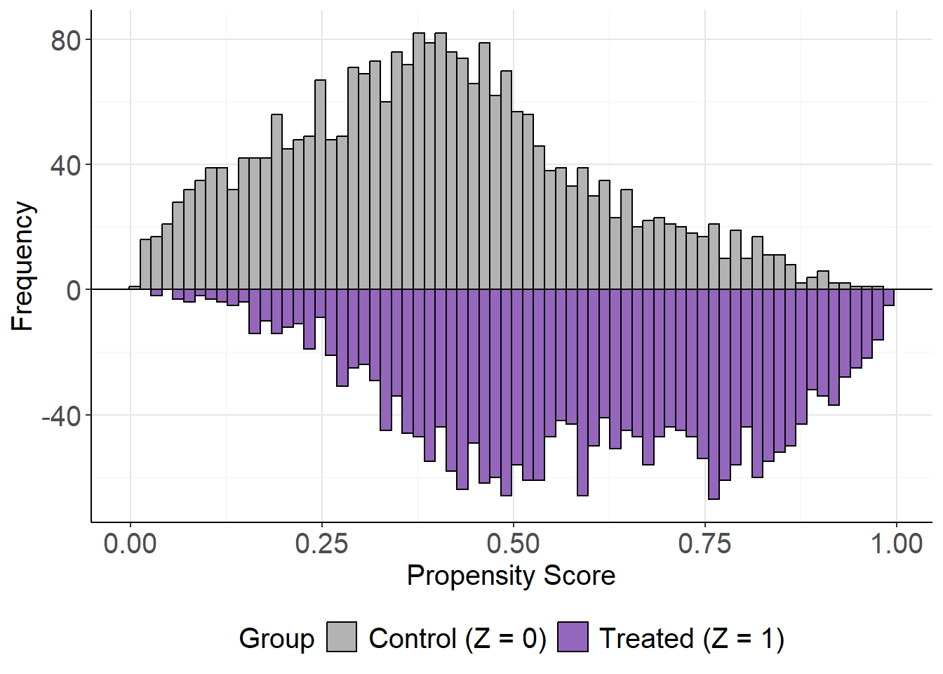
# Mirror histogram for covariate distribution balance
mirror_hist(lbc_net.fit)
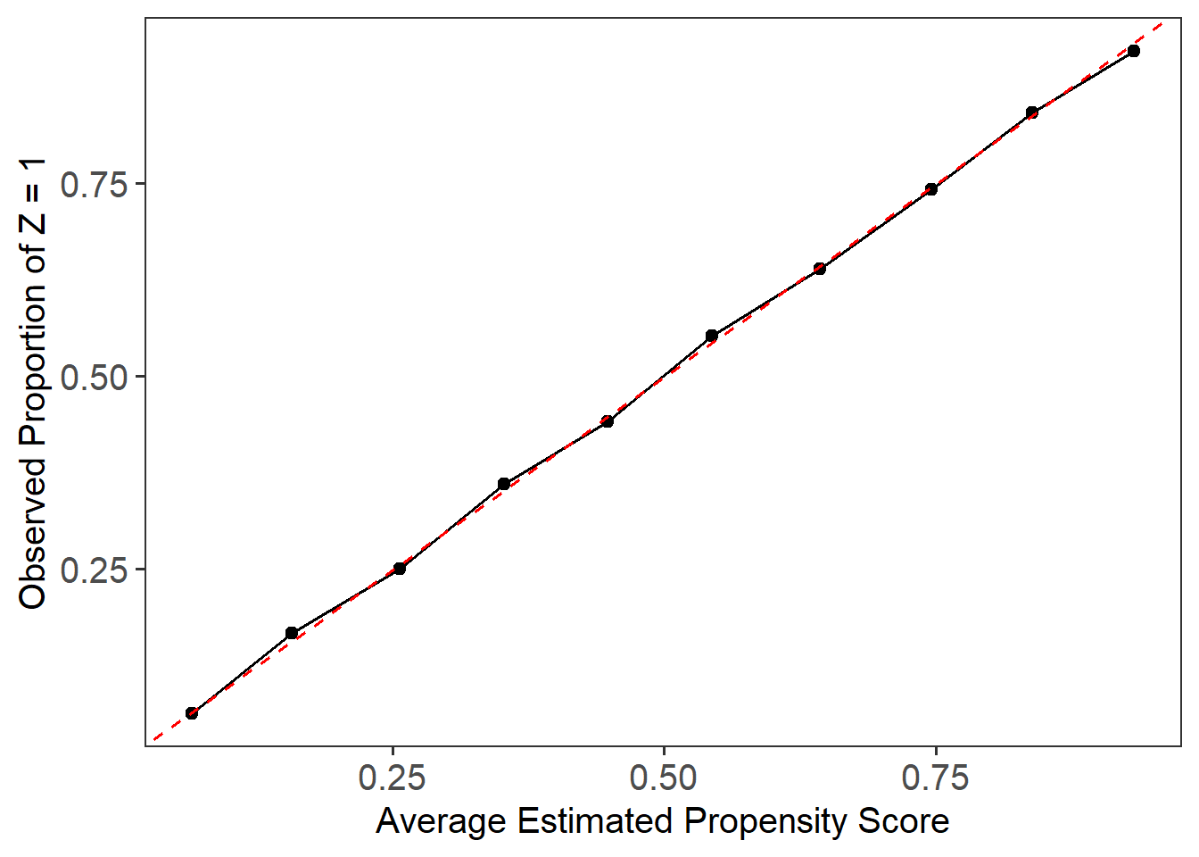
# Calibration plot to assess model calibration
plot_calib(lbc_net.fit)
Evaluate Covariate Balance
# Compute local balance diagnostics
lsd.fit <- lsd(lbc_net.fit)

# Print and summarize local balance
print(lsd.fit)
Sample Size: 5000  | Treated: 2466  | Control: 2534
Estimand: ATE (Average Treatment Effect)

--- Local Balance (LSD) % ---
Max LSD: 3.9246
Mean LSD: 0.4018

Kernel: "gaussian"

Use summary(object) for a full model summary.
Call:
 function (x, ...)  UseMethod("formula")
Sample Size: 5000  | Number of Covariates: 4
Treated: 2466  | Control: 2534
Estimand: ATE (Average Treatment Effect)

--- Local Balance (LSD) % ---
Max LSD:   3.9246
Mean LSD:  0.4018

Covariates   LSD %
-------------
X1    0.8687
X2    0.3959
X3    0.1678
X4    0.1749
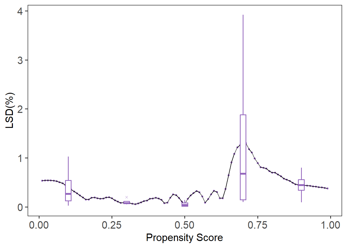
# Plot local balance metrics
plot(lsd.fit)
For a more detailed tutorial, visit our Step-by-Step Tutorial.